Lab 9
Probability (II)
Continuous Random Variable (RV)
While a discrete random variable only takes distinct values, a continuous random variable can take any value within its given range. For example, it might yield a value between 10 and 120 (such as the daily high temperature in the U.S.) or any value from 0 to infinity (such as the failure time of a particular device in minutes).
Probability Distribution of Continuous RV
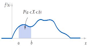
A continuous probability distribution can be represented as a curve \(f(x)\) that spans the possible values of a random variable. Its shape can vary depending on the variable of interest, but it has the following properties:
- \(f(x)\ge 0\) for all \(x\);
- The total area under the probability density curve is always 1;
- \(P[ a\le X\le b ]\) is the area under the probability density curve between \(a\) and \(b\).
The Normal Distribution
In class, we primarily focus on the normal distribution because:
- Many real-world phenomena follow a normal distribution, such as people’s height, IQ scores, exam grades, snowflake sizes, measurement errors, and lightbulb lifetimes.
- The Central Limit Theorem ensures that sums and averages of independent random variables tend to be normally distributed.
- The normal distribution is mathematically convenient and easy to work with. In particular, we can always use \(z\)-table for any probability calculations.
A normal distribution can be characterized by two parameters: the mean \(\mu\) and the variance \(\sigma^2\) (or equivalently, the standard deviation \(\sigma\)).

Probability calculation
Probability calculations under a normal distribution can be easily performed using the function \(\texttt{\color{brown}{pnorm(c)}}\). Similar to using a \(z\)-table, this function provides the left-tail probability based on a cutoff value of \(c\).
Suppose \(X\) to be the # of beer cans consumed by a female college student in a year. It is assumed to be normally distributed with the mean 260 and standard deviation 80. What we are interested in is the proportion of female students drink less than 300 beer cans per year.
This approach precisely emulates the way we typically perform probability calculations using the \(z\)-table. Now, we can simplify the process by using the second and third arguments of the \(\texttt{\color{brown}{pnorm()}}\) function, which allow us to specify the mean and standard deviation of the distribution directly.
Example
Let \(Y\) be the # of beer cans consumed by a male college student in a year. It is assumed to be normally distributed with the mean 440 and standard deviation 60. What proportion of male students drink more than 365 beer cans per year?
Sampling Distribution for Sample Mean
The sampling distribution contains all the information about a statistic of interest. When examining the behavior of a sample mean randomly drawn from a population, we first consider the following properties:
- The mean of “the sampling distribution for the sample mean” will always equal the population mean \(\mu\): \[\mu_\bar{X}=E[\bar{X}]=\mu.\]
- The standard deviation of “the sampling distribution for the sample mean” will equal the population standard deviation \(\sigma\) over the square root of the sample size \(n\): \[\sigma_\bar{X}=SD[\bar{X}]=\frac{\sigma}{\sqrt{n}}.\]
Then, the shape of the sampling distribution can be described as follows:
If population distribution is a normal distribution, the sampling distribution for sample mean would resemble the shape of the population distribution. That is, the sampling distribution also follows a normal distribution with the above mean and standard deviation.
If population distribution is unknown, the sampling distribution for sample mean would still follow a normal distribution with the above mean and standard deviation only if we have sufficiently large sample size, e.g., \(n\ge 30\).
In particular, we call the second result the central limit theorem (C.L.T.).
Probability calculation
Suppose a test score has the mean value 78 and standard deviation 10. We don’t have any other information regarding the population distribution. Let us consider the probability that a sample mean with the sample size \(n=32\) is greater than 82, i.e., the probability that the average test score of 32 students is greater than 82.
Note that if the sample size were smaller than 30, the probability calculation would be impossible since the appropriate probability distribution for the computation would be unknown.
Verification of C.L.T. through a simulation
Lastly, let us verify the central limit theorem through a short simulation. Here, we assume the population distribution is highly skewed to the right.
Note that the shape of the histogram (the empirical sample mean distribution) converges toward the theoretical sampling distribution (represented by the black curve) as the sample size increases from \(n=2\) to \(n=30\).
Lab Questions
- A survey indicates that the average American family produces 17.2 pounds of glass waste per year, with a population standard deviation of 2.5 pounds. Calculate the probability that the sample mean for a group of 55 families will fall between 17 and 18 pounds.
Can we use the C.L.T. for the probability calculation?
True / FalseCalculate the probability.
- The average teacher’s salary in New Jersey is $62,174, assuming a normal distribution with a standard deviation of $8,500.
- What is the probability that a randomly selected teacher makes less than $60,000 per year?
- If we sample 100 teachers’ salaries, what is the probability that the sample mean is less than $60,000 per year?
- Why is the probability in part (i) higher than the probability in part (ii)?
Click HERE to submit your answers.